Metabolite compound name transformation
Metabolite compound name transform to RefMet name
This step requires networking
RefMet: A Reference list of Metabolite names.The main objective of RefMet is to provide a standardized reference nomenclature for both discrete metabolite structures and metabolite species identified by spectroscopic techniques in metabolomics experiments.
library(MNet)
library(dplyr)
library(tibble)
library(survival)
library(tidyr)
library(knitr)
library(stringr)
library(ggplot2)
library(RColorBrewer)
library(clusterProfiler)
library(org.Hs.eg.db)
library(pathview)
compound_name <- c("2-Hydroxybutyric acid",
                   "1-Methyladenosine",
                   "tt",
                   "2-Aminooctanoic acid")
## transform the compound name to refmet name
refmetid_result <- name2refmet(compound_name)
head(refmetid_result)
## Input_name Refmet_name Formula Super_class
## 1 2-Hydroxybutyric acid 2-Hydroxybutyric acid C4H8O3 Fatty Acyls
## 2 1-Methyladenosine 1-Methyladenosine C11H15N5O4 Nucleic acids
## 3 tt tt - -
## 4 2-Aminooctanoic acid 2-Aminocaprylic acid C8H17NO2 Fatty Acyls
## Main_class Sub_class
## 1 Fatty acids Hydroxy FA
## 2 Purines Purine ribonucleosides
## 3 - -
## 4 Fatty acids Amino FAMetabolite compound name transform to KEGG ID
This step requires networking
Transform the metabolites compound name to KEGG ID
compound_name <- c("2-Hydroxybutyric acid",
                   "1-Methyladenosine",
                   "tt",
                   "2-Aminooctanoic acid")
## transform the compound name to KEGG ID, some metabolites have several KEGG ID
keggid_result <- name2keggid(compound_name) %>%
  separate_rows(KEGG_id, sep = ";")
head(keggid_result)
## # A tibble: 4 × 2
## Name KEGG_id
## <chr> <chr>
## 1 2-Hydroxybutyric acid C05984
## 2 1-Methyladenosine C02494
## 3 tt NA
## 4 2-Aminooctanoic acid NAMetabolite name corresponding to kegg pathway
This step requires networking
Search the kegg pathway corresponding to the metabolite name
compound_name <- c("2-Hydroxybutyric acid",
"1-Methyladenosine",
"tt",
"2-Aminooctanoic acid")
## Search the kegg pathway corresponding to the metabolite name
result_all <- name2pathway(compound_name)
head(result_all)## $name2pathway
## # A tibble: 1 × 5
## Name KEGG_id Pathway Pathway_category Pathway_id
## <chr> <chr> <chr> <chr> <chr>
## 1 2-Hydroxybutyric acid C05984 Propanoate metaboli… Carbohydrate me… hsa00640
##
## $pathway
## # A tibble: 1 × 16
## name nAnno nOverlap fc zscore pvalue adjp or CIl CIu distance
## <chr> <dbl> <dbl> <dbl> <dbl> <dbl> <dbl> <dbl> <dbl> <dbl> <chr>
## 1 Propanoat… 40 1 76.1 8.66 0 0 Inf 1.93 Inf 1
## # ℹ 5 more variables: namespace <chr>, members_Overlap <chr>,
## # members_Anno <chr>, members_Overlap_name <chr>, members_Anno_name <chr>
##
## $kegg_id
## # A tibble: 4 × 2
##   Name                  KEGG_id
##   <chr>                 <chr>
## 1 2-Hydroxybutyric acid C05984
## 2 1-Methyladenosine     C02494
## 3 tt                    NA
## 4 2-Aminooctanoic acid  NA
##### Output is the each metabolite related pathway
result_name2pathway <- result_all$name2pathway
head(result_name2pathway)
## # A tibble: 1 × 5
## Name KEGG_id Pathway Pathway_category Pathway_id
## <chr> <chr> <chr> <chr> <chr>
## 1 2-Hydroxybutyric acid C05984 Propanoate metaboli… Carbohydrate me… hsa00640
## the KEGG ID of the metabolite name
result_name2keggid <- result_all$kegg_id
head(result_name2keggid)
## # A tibble: 4 × 2
## Name KEGG_id
## <chr> <chr>
## 1 2-Hydroxybutyric acid C05984
## 2 1-Methyladenosine C02494
## 3 tt NA
## 4 2-Aminooctanoic acid NA
## the pathway of the metabolite name
result_name2enrichpathway <- result_all$pathway
head(result_name2enrichpathway)
## # A tibble: 1 × 16
## name nAnno nOverlap fc zscore pvalue adjp or CIl CIu distance
## <chr> <dbl> <dbl> <dbl> <dbl> <dbl> <dbl> <dbl> <dbl> <dbl> <chr>
## 1 Propanoat… 40 1 76.1 8.66 0 0 Inf 1.93 Inf 1
## # ℹ 5 more variables: namespace <chr>, members_Overlap <chr>,
## # members_Anno <chr>, members_Overlap_name <chr>, members_Anno_name <chr>Metabolite KEGG ID transform to KEGG pathway
KEGG ID transform to KEGG pathway
keggid <- c("C05984", "C02494")
##### the output is the each metabolite related pathway
keggpathway_result <- keggid2pathway(keggid)
head(keggpathway_result)
## # A tibble: 1 × 5
## ENTRY NAME PATHWAY pathway_type V2
## <chr> <chr> <chr> <chr> <chr>
## 1 C05984 2-Hydroxybutanoic acid;///2-Hydroxybutyrate… Propan… Carbohydrat… hsa0…Pathway information
Get the gene and the metabolite in the pathway
## the genes and metabolites in pathway 'hsa00630'
result <- pathwayinfo("hsa00630")

## the genes and metabolites in pathway 'Glyoxylate and dicarboxylate metabolism'
result <- pathwayinfo("Glyoxylate and dicarboxylate metabolism")

head(result$gene_info[1:2, ])
## type name kegg_pathwayid kegg_pathwayname
## 1 gene ACSS1 hsa00630 Glyoxylate and dicarboxylate metabolism
## 2 gene ACSS2 hsa00630 Glyoxylate and dicarboxylate metabolism
## kegg_category
## 1 Carbohydrate metabolism
## 2 Carbohydrate metabolism
head(result$compound_info[1:2, ])## type name kegg_pathwayid kegg_pathwayname
## 1 metabolite C00007 hsa00630 Glyoxylate and dicarboxylate metabolism
## 2 metabolite C00011 hsa00630 Glyoxylate and dicarboxylate metabolism
## kegg_category
## 1 Carbohydrate metabolism
## 2 Carbohydrate metabolismPathway name transform to pathway id
Transform the KEGG pathway name to KEGG pathway ID
## the KEGG pathway ID of pathway name
pathwayid <- pathway2pathwayid("Glycolysis / Gluconeogenesis")
head(pathwayid)
## PATHWAY pathwayid
## 1 Glycolysis / Gluconeogenesis hsa00010Group-wise analyses
Differnetial metabolite analysis
Function ‘mlimma’
## mlimma is the function of Differential Metabolite analysis by limma
diff_result <- mlimma(meta_dat, group)
head(diff_result)
## # A tibble: 6 × 8
## logFC AveExpr t P.Value adj.P.Val B logP name
## <dbl> <dbl> <dbl> <dbl> <dbl> <dbl> <dbl> <chr>
## 1 2.86 22.6 9.25 1.52e-10 0.0000000332 14.1 7.48 C02045
## 2 2.44 26.2 7.80 6.83e- 9 0.000000748 10.4 6.13 C00267
## 3 -1.82 27.1 -6.80 1.10e- 7 0.00000622 7.64 5.21 C00073
## 4 -3.78 20.9 -6.79 1.14e- 7 0.00000622 7.61 5.21 C05674
## 5 -2.20 21.4 -6.58 2.07e- 7 0.00000907 7.02 5.04 C00255
## 6 -2.37 21.6 -6.45 2.98e- 7 0.0000109 6.66 4.96 C00242Function ‘DM’
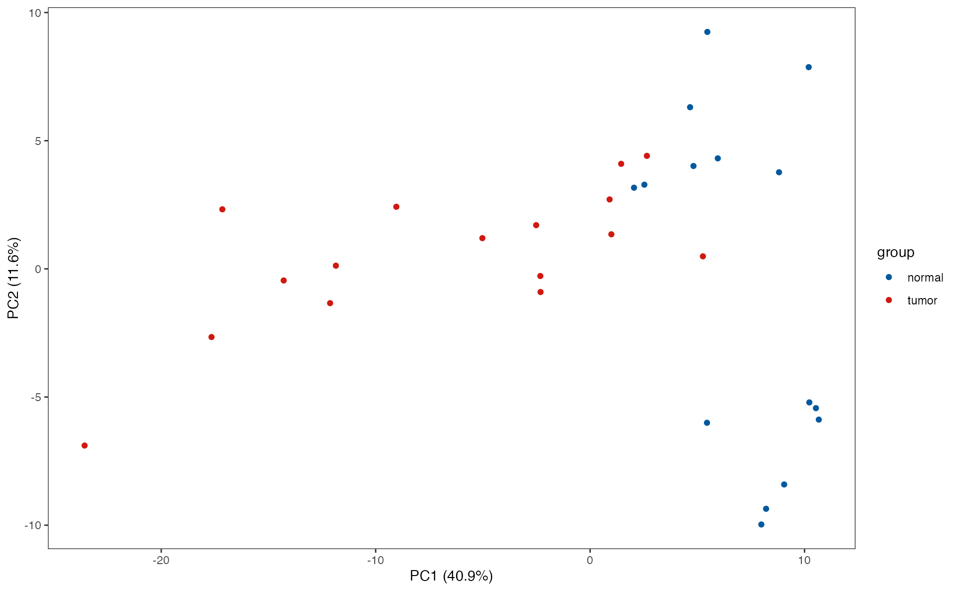
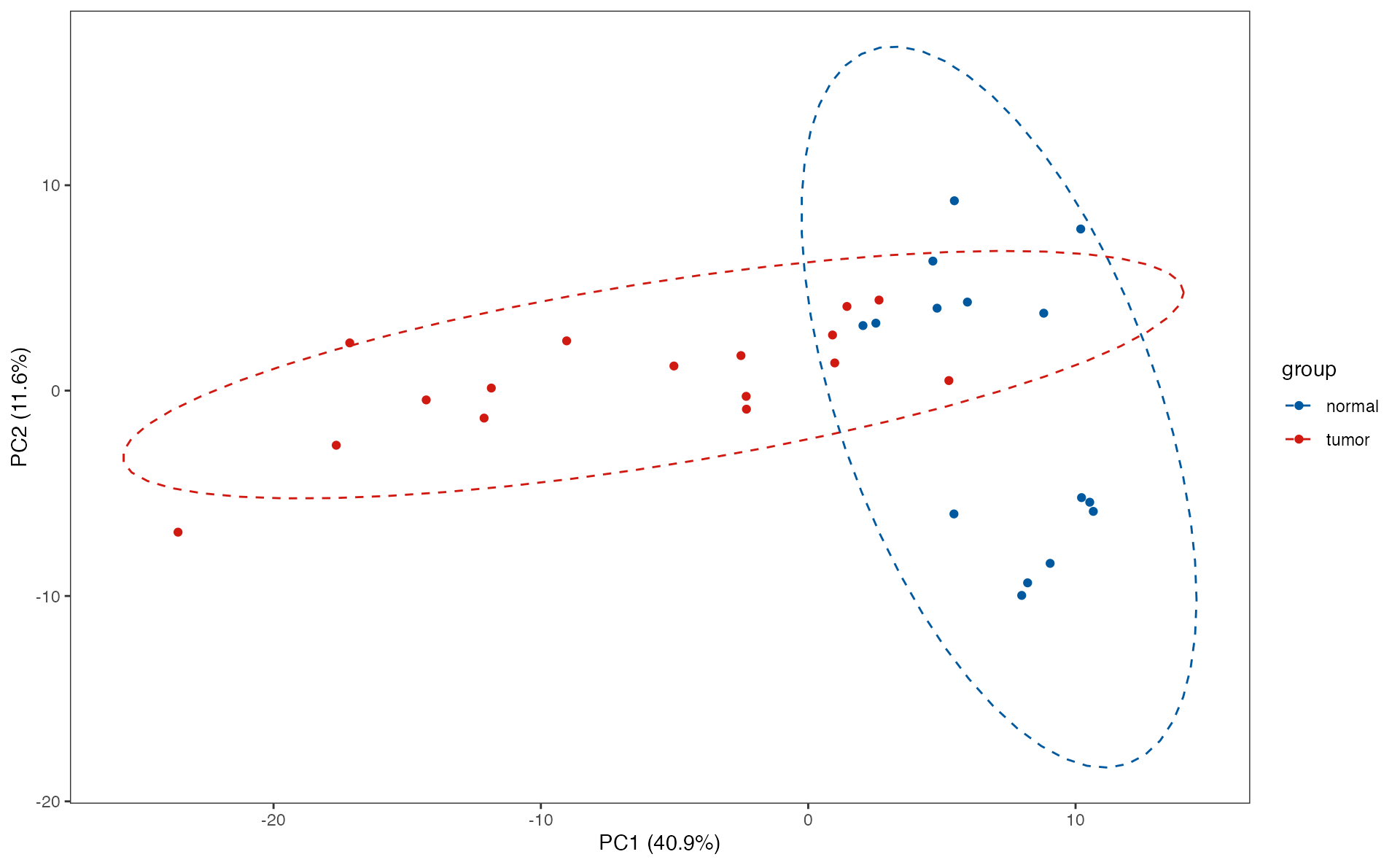
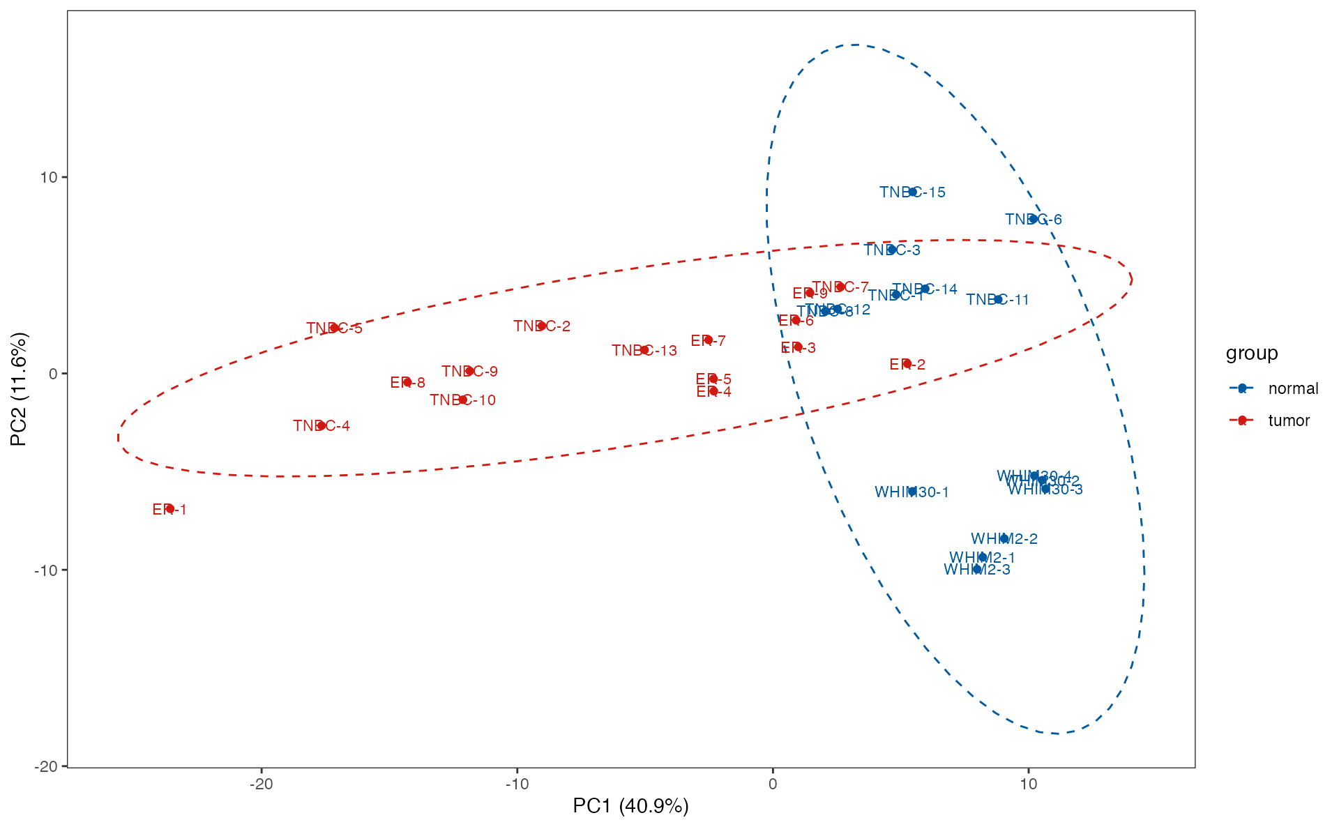
## DM is the function of Differential Metabolite analysis by OPLS-DA
diff_result <- DM(2 ** meta_dat, group)
## OPLS-DA
## 31 samples x 219 variables and 1 response
## standard scaling of predictors and response(s)
## R2X(cum) R2Y(cum) Q2(cum) RMSEE pre ort pR2Y pQ2
## Total 0.485 0.864 0.697 0.194 1 1 0.05 0.05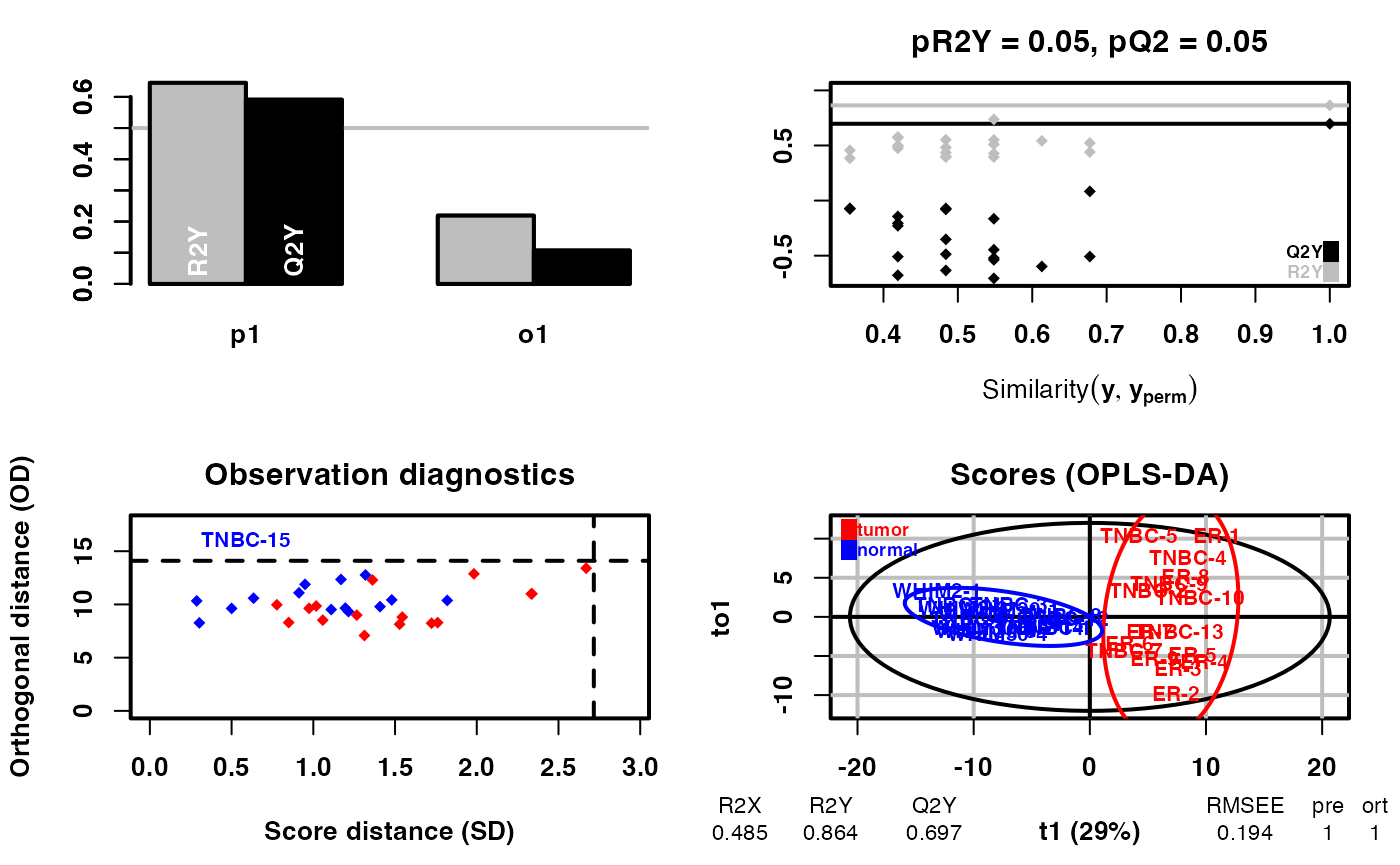
head(diff_result)## # A tibble: 6 × 7
## Name Fold_change PValue_t Padj_t PValue_wilcox Padj_wilcox VIP
## <chr> <dbl> <dbl> <dbl> <dbl> <dbl> <dbl>
## 1 C09642 0.842 0.168 0.221 0.173 0.224 0.520
## 2 C05581 0.402 0.000793 0.00220 0.00192 0.00494 1.12
## 3 C03264 0.434 0.0000617 0.000338 0.000187 0.000855 1.33
## 4 C15025 0.683 0.00266 0.00614 0.00763 0.0165 0.995
## 5 C00408 1.63 0.00688 0.0142 0.0187 0.0359 1.03
## 6 C02918 0.497 0.677 0.734 0.0855 0.125 0.0628
## filter the differential metabolites by default fold change >1.3 or < 1/1.3 ,fdr < 0.05 and VIP>0.8

diff_result_filter <- diff_result %>%
  filter(Fold_change > 1.3 | Fold_change < 1 / 1.3) %>%
  filter(Padj_wilcox < 0.1) %>%
  filter(VIP > 0.8)
head(diff_result_filter)
## # A tibble: 6 × 7
## Name Fold_change PValue_t Padj_t PValue_wilcox Padj_wilcox VIP
## <chr> <dbl> <dbl> <dbl> <dbl> <dbl> <dbl>
## 1 C05581 0.402 0.000793 0.00220 0.00192 0.00494 1.12
## 2 C03264 0.434 0.0000617 0.000338 0.000187 0.000855 1.33
## 3 C15025 0.683 0.00266 0.00614 0.00763 0.0165 0.995
## 4 C00408 1.63 0.00688 0.0142 0.0187 0.0359 1.03
## 5 C06178 0.397 0.0000155 0.000121 0.0000839 0.000510 1.41
## 6 C02220 0.452 0.0403 0.0631 0.0552 0.0876 0.983Differential metabolites’ volcano
Volcano plot of metabolites using the function “pVolcano”
p_volcano <- pVolcano(diff_result, foldchange_threshold = 1.5)## [1] 1.5
p_volcano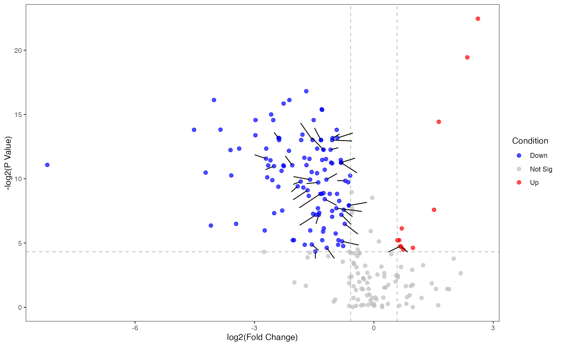
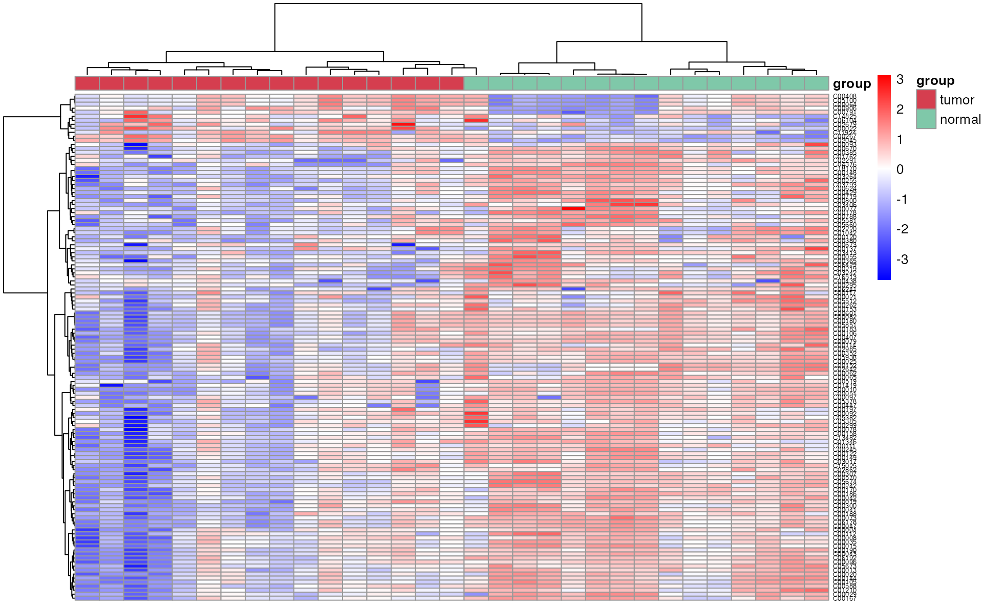
Differential metabolites’ heatmap
Heatmap plot of differentital metabolites using the function “pHeatmap”
meta_dat_diff <- meta_dat[rownames(meta_dat) %in% diff_result_filter$Name, ]
p_heatmap <- pHeatmap(
  meta_dat_diff,
  group,
  fontsize_row = 5,
  fontsize_col = 4,
  clustering_method = "ward.D",
  clustering_distance_cols = "correlation"
)
Differential metabolites’ zscore
Zscore plot of differentital metabolites using the function “pZscore”
p_zscore <- pZscore(meta_dat_diff, group, ysize = 3)
p_zscore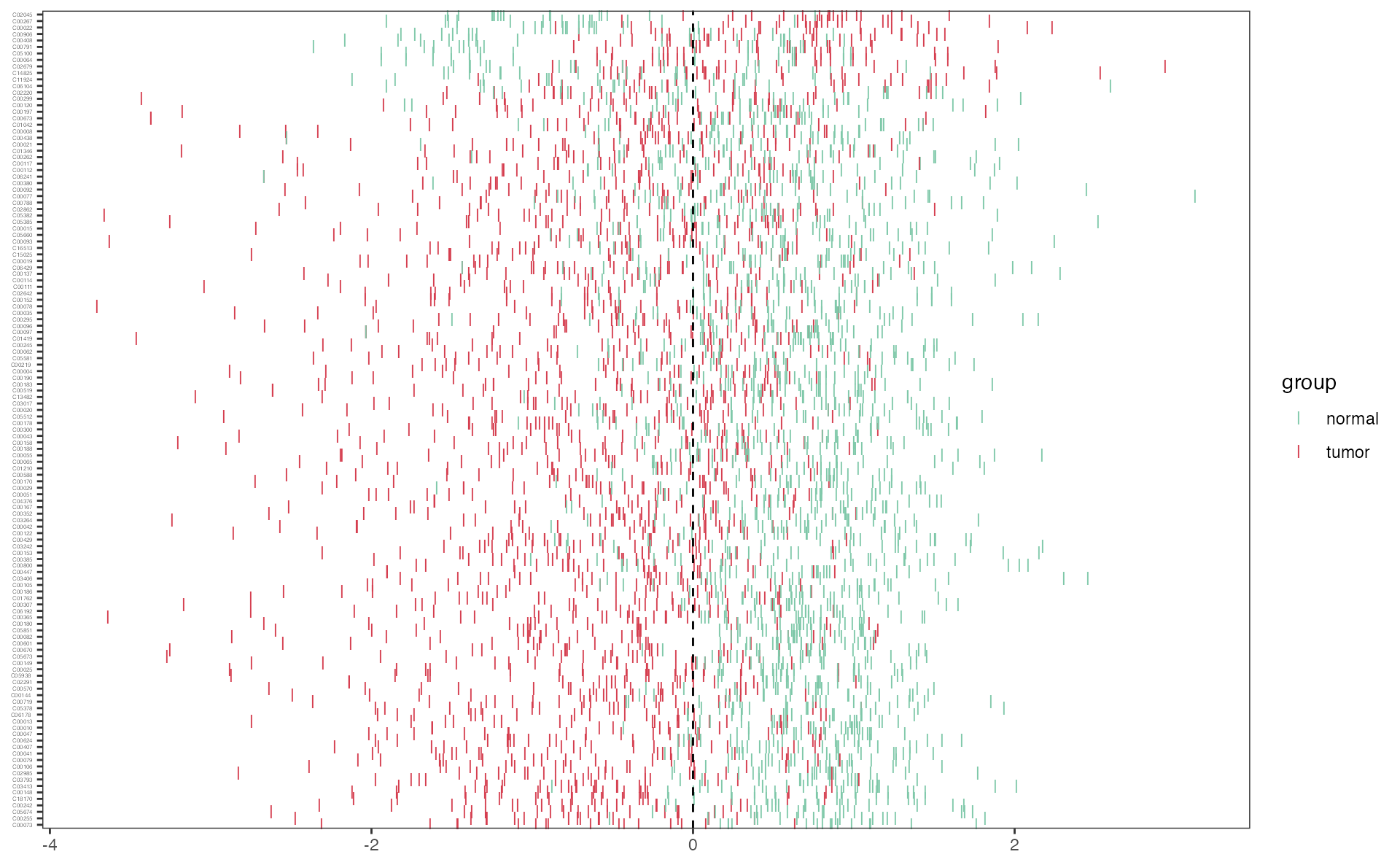
Feature selection
Boruta
Using machine learning “Boruta” for feature selection
#group <- rep("normal",length(names(meta_dat)))
#group[grep("TUMOR",names(meta_dat))] <- "tumor"
meta_dat1 <- t(meta_dat) %>%
  as.data.frame() %>%
  mutate(group = group)

result_ML_Boruta <- ML_Boruta(meta_dat1)
head(result_ML_Boruta)
## name meanImp medianImp minImp maxImp normHits decision
## 1 C03264 1.807909 1.890535 -1.00100150 3.192239 0.6052104 Confirmed
## 2 C02630 3.904201 3.907530 2.23148770 5.273588 1.0000000 Confirmed
## 3 C00170 2.320137 2.383305 0.03629764 3.677534 0.8496994 Confirmed
## 4 C18170 3.504635 3.485503 1.99657024 4.950293 0.9979960 Confirmed
## 5 C06192 2.226020 2.252420 -0.15535207 3.605125 0.8136273 Confirmed
## 6 C00267 4.249434 4.265181 2.71962194 5.732876 1.0000000 ConfirmedRandom Forest
Using machine learning “Random Forest” for feature selection
result_ML_RF <- ML_RF(meta_dat1)
result_ML_RF$p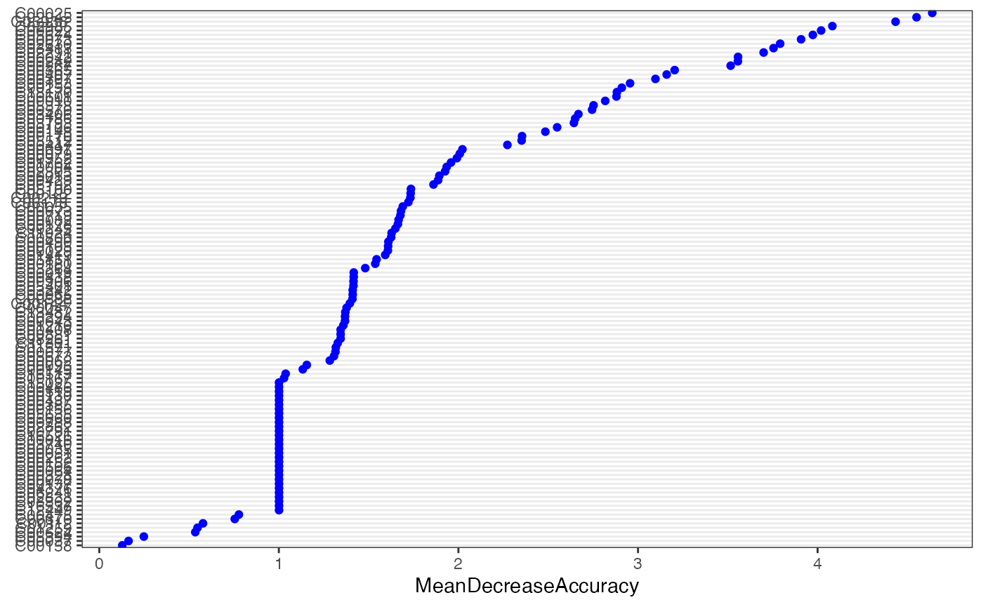
result_ML_RF$feature_result## # A tibble: 122 × 6
## normal tumor MeanDecreaseAccuracy MeanDecreaseGini names raw
## <dbl> <dbl> <dbl> <dbl> <chr> <fct>
## 1 4.23 4.04 4.64 0.548 C00025 C00025
## 2 4.34 4.22 4.55 0.561 C02045 C02045
## 3 4.38 3.67 4.43 0.527 C05938. C05938
## 4 3.58 3.79 4.08 0.470 C02985 C02985
## 5 4.22 3.35 4.02 0.517 C00022 C00022
## 6 3.41 3.77 3.97 0.458 C05674 C05674
## 7 3.55 3.89 3.91 0.452 C00073 C00073
## 8 3.90 2.62 3.79 0.415 C02630 C02630
## 9 3.70 3.26 3.75 0.368 C03413 C03413
## 10 3.45 3.40 3.70 0.390 C02291 C02291
## # ℹ 112 more rowsXGBoost
Using machine learning ” XGBoost” for feature selection
result_ML_xgboost <- ML_xgboost(meta_dat1)## [1] train-rmse:0.364289 test-rmse:0.549992
## [2] train-rmse:0.265516 test-rmse:0.535074
## [3] train-rmse:0.193648 test-rmse:0.536247
## [4] train-rmse:0.141421 test-rmse:0.518435
## [5] train-rmse:0.103574 test-rmse:0.539353
## [6] train-rmse:0.076240 test-rmse:0.517378
## [7] train-rmse:0.056624 test-rmse:0.509748
## [8] train-rmse:0.042572 test-rmse:0.506916
## [9] train-rmse:0.032249 test-rmse:0.499201
## [10] train-rmse:0.024705 test-rmse:0.498236
## [11] train-rmse:0.019147 test-rmse:0.500697
## [12] train-rmse:0.014733 test-rmse:0.502704
## [13] train-rmse:0.011439 test-rmse:0.504271
## [14] train-rmse:0.009015 test-rmse:0.505542
## [15] train-rmse:0.007161 test-rmse:0.506894
## [16] train-rmse:0.005807 test-rmse:0.507730
## [17] train-rmse:0.004745 test-rmse:0.508582
## [18] train-rmse:0.003928 test-rmse:0.509305
## [19] train-rmse:0.003291 test-rmse:0.510078
## [20] train-rmse:0.002775 test-rmse:0.510652
## [21] train-rmse:0.002346 test-rmse:0.510730
## [22] train-rmse:0.002007 test-rmse:0.510676
## [23] train-rmse:0.001711 test-rmse:0.511044
## [24] train-rmse:0.001457 test-rmse:0.511389
## [25] train-rmse:0.001240 test-rmse:0.511672
## [26] train-rmse:0.001068 test-rmse:0.511877
## [27] train-rmse:0.000922 test-rmse:0.512052
## [28] train-rmse:0.000799 test-rmse:0.512173
## [29] train-rmse:0.000688 test-rmse:0.512132
## [30] train-rmse:0.000592 test-rmse:0.512268
## [31] train-rmse:0.000530 test-rmse:0.512363
## [32] train-rmse:0.000481 test-rmse:0.512445
## [33] train-rmse:0.000441 test-rmse:0.512502
## [34] train-rmse:0.000406 test-rmse:0.512478
## [35] train-rmse:0.000374 test-rmse:0.512488
## [36] train-rmse:0.000374 test-rmse:0.512490
## [37] train-rmse:0.000374 test-rmse:0.512491
## [38] train-rmse:0.000374 test-rmse:0.512492
## [39] train-rmse:0.000374 test-rmse:0.512493
## [40] train-rmse:0.000374 test-rmse:0.512493
## [41] train-rmse:0.000374 test-rmse:0.512493
## [42] train-rmse:0.000374 test-rmse:0.512494
## [43] train-rmse:0.000374 test-rmse:0.512494
## [44] train-rmse:0.000374 test-rmse:0.512494
## [45] train-rmse:0.000374 test-rmse:0.512494
## [46] train-rmse:0.000374 test-rmse:0.512494
## [47] train-rmse:0.000374 test-rmse:0.512494
## [48] train-rmse:0.000374 test-rmse:0.512494
## [49] train-rmse:0.000374 test-rmse:0.512494
## [50] train-rmse:0.000374 test-rmse:0.512494
## [51] train-rmse:0.000374 test-rmse:0.512494
## [52] train-rmse:0.000374 test-rmse:0.512494
## [53] train-rmse:0.000374 test-rmse:0.512494
## [54] train-rmse:0.000374 test-rmse:0.512494
## [55] train-rmse:0.000374 test-rmse:0.512494
## [56] train-rmse:0.000374 test-rmse:0.512494
## [57] train-rmse:0.000374 test-rmse:0.512494
## [58] train-rmse:0.000374 test-rmse:0.512494
## [59] train-rmse:0.000374 test-rmse:0.512494
## [60] train-rmse:0.000374 test-rmse:0.512494
## [61] train-rmse:0.000374 test-rmse:0.512494
## [62] train-rmse:0.000374 test-rmse:0.512494
## [63] train-rmse:0.000374 test-rmse:0.512494
## [64] train-rmse:0.000374 test-rmse:0.512494
## [65] train-rmse:0.000374 test-rmse:0.512494
## [66] train-rmse:0.000374 test-rmse:0.512494
## [67] train-rmse:0.000374 test-rmse:0.512494
## [68] train-rmse:0.000374 test-rmse:0.512494
## [69] train-rmse:0.000374 test-rmse:0.512494
## [70] train-rmse:0.000374 test-rmse:0.512494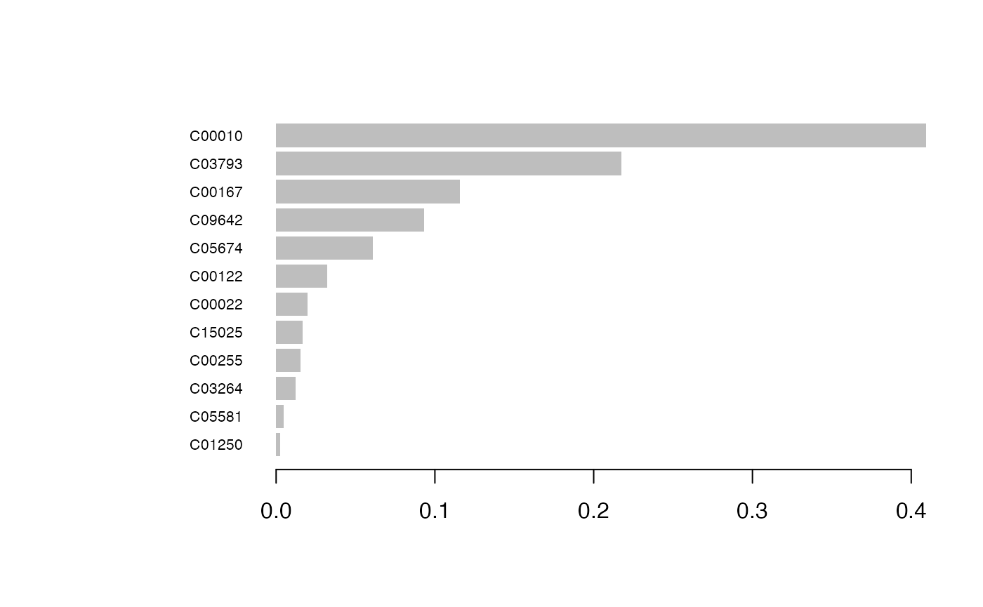
result_ML_xgboost$p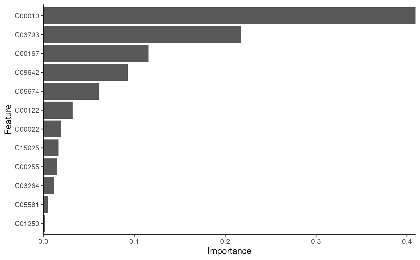
result_ML_xgboost$feature_result## Feature Gain Cover Frequency Importance
## <fctr> <num> <num> <num> <num>
## 1: C00010 0.409537590 0.05868545 0.04347826 0.409537590
## 2: C03793 0.217514348 0.05868545 0.04347826 0.217514348
## 3: C00167 0.115622639 0.05868545 0.04347826 0.115622639
## 4: C09642 0.093095188 0.15258216 0.21739130 0.093095188
## 5: C05674 0.060828633 0.05868545 0.04347826 0.060828633
## 6: C00122 0.032337968 0.05868545 0.04347826 0.032337968
## 7: C00022 0.019764628 0.11737089 0.08695652 0.019764628
## 8: C15025 0.016607794 0.03051643 0.04347826 0.016607794
## 9: C00255 0.015274112 0.17605634 0.13043478 0.015274112
## 10: C03264 0.012220371 0.09859155 0.13043478 0.012220371
## 11: C05581 0.004831088 0.03286385 0.04347826 0.004831088
## 12: C01250 0.002365641 0.09859155 0.13043478 0.002365641LASSO
Using machine learning “LASSO” for feature selection
##      feature         s1
## 1 `C01879  ` -0.2834664
## 2     C00010 -0.1512106
## 3     C02291 -0.1897965
## 4     C02045  1.1011873
## 5     C00073 -0.3605763
## 6 C00065 -0.2661594Pathway analysis
Pathview only metabolites
kegg_id <- c("C02494", "C03665", "C01546", "C05984", "C14088", "C00587")
value <- c(-0.3824620,
           0.1823628,
           -1.1681486,
           0.5164899,
           1.6449798,
           -0.7340652)
names(value) <- kegg_id
cpd.data <- value

gene_name <- c("LDHA", "BCKDHB", "PCCA", "ACSS1")
gene_value <- c(1, 0.5, -1, -1)
names(gene_value) <- gene_name

## pathview plot of metabolites
pPathview(cpd.data, outdir = "result_v0131")
Pathview contains metabolites and genes
## pathview plot of genes and metabolites
pPathview(cpd.data = cpd.data,
          gene.data = gene_value,
          outdir = "result_v0131")
Clinical analysis
Time series of clinical
Column contains the time, group, clinical index(such as ALT), low and high
clinical_index[1:5, ]## time group ALT low high
## 1 1 B 13 10 64
## 2 2 B 13 10 64
## 3 3 B 14 10 64
## 4 4 B 24 10 64
## 5 5 B 255 10 64
time_series_ALT <- pCliTS(clinical_index, "ALT")
time_series_ALT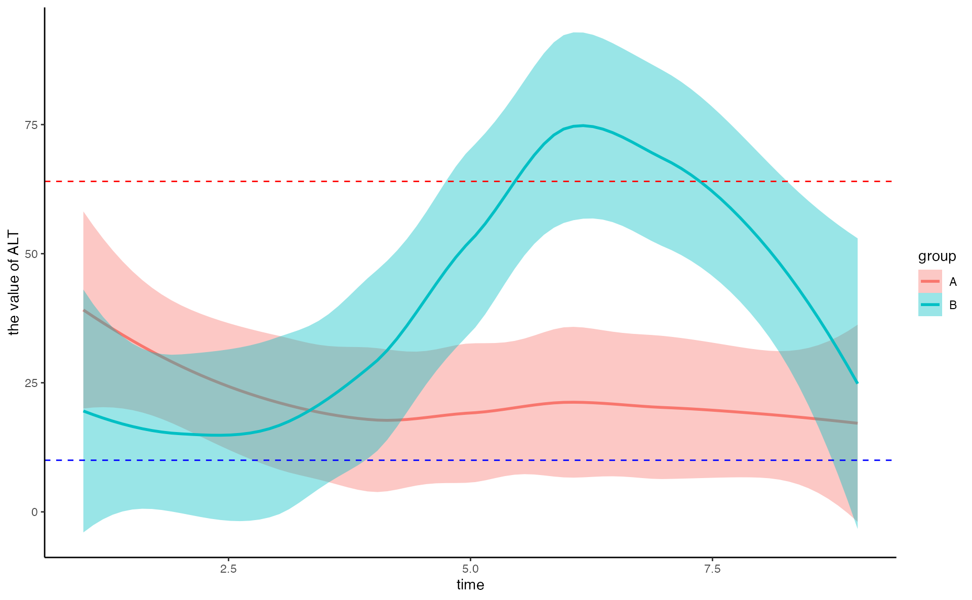
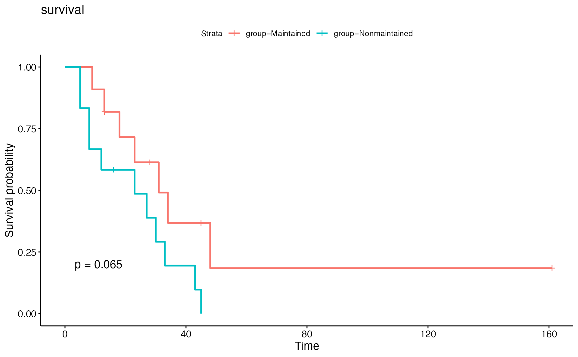
Cox analysis
## # A tibble: 6 × 5
##   name   beta     `HR (95% CI for HR)` wald.test p.value
##   <chr>  <chr>    <chr>                <chr>     <chr>
## 1 C03819 1.2e-06  1 (1-1)              0.31      0.58
## 2 C02918 4.8e-07  1 (1-1)              0.1       0.75
## 3 C03916 -1.7e-07 1 (1-1)              0.11      0.74
## 4 C04102 -3.1e-08 1 (1-1)              0.07      0.79
## 5 C01885 6.3e-07  1 (1-1)              0.12      0.73
## 6 C07326 -5.1e-06 1 (1-1)              0.22      0.64
Session information
## R version 4.4.2 (2024-10-31)
## Platform: x86_64-apple-darwin20
## Running under: macOS Ventura 13.7.1
##
## Matrix products: default
## BLAS:   /Library/Frameworks/R.framework/Versions/4.4-x86_64/Resources/lib/libRblas.0.dylib
## LAPACK: /Library/Frameworks/R.framework/Versions/4.4-x86_64/Resources/lib/libRlapack.dylib;  LAPACK version 3.12.0
##
## locale:
## [1] en_US.UTF-8/en_US.UTF-8/en_US.UTF-8/C/en_US.UTF-8/en_US.UTF-8
##
## time zone: Asia/Shanghai
## tzcode source: internal
##
## attached base packages:
## [1] stats4    stats     graphics  grDevices utils     datasets  methods
## [8] base
##
## other attached packages:
##  [1] caret_6.0-94           lattice_0.22-6         pathview_1.46.0
##  [4] org.Hs.eg.db_3.20.0    AnnotationDbi_1.68.0   IRanges_2.40.0
##  [7] S4Vectors_0.44.0       Biobase_2.66.0         BiocGenerics_0.52.0
## [10] clusterProfiler_4.14.1 RColorBrewer_1.1-3     ggplot2_3.5.1
## [13] stringr_1.5.1          knitr_1.49             tidyr_1.3.1
## [16] survival_3.7-0         tibble_3.2.1           dplyr_1.1.4
## [19] MNet_1.2.0
##
## loaded via a namespace (and not attached):
##   [1] fs_1.6.5                    matrixStats_1.4.1
##   [3] bitops_1.0-9                enrichplot_1.26.2
##   [5] lubridate_1.9.3             httr_1.4.7
##   [7] Rgraphviz_2.50.0            tools_4.4.2
##   [9] backports_1.5.0             utf8_1.2.4
##  [11] R6_2.5.1                    mgcv_1.9-1
##  [13] lazyeval_0.2.2              withr_3.0.2
##  [15] gridExtra_2.3               cli_3.6.3
##  [17] textshaping_0.4.0           labeling_0.4.3
##  [19] sass_0.4.9                  KEGGgraph_1.66.0
##  [21] filesstrings_3.4.0          survMisc_0.5.6
##  [23] readr_2.1.5                 randomForest_4.7-1.2
##  [25] proxy_0.4-27                pkgdown_2.1.1
##  [27] yulab.utils_0.1.8           systemfonts_1.1.0
##  [29] gson_0.1.0                  foreign_0.8-87
##  [31] DOSE_4.0.0                  R.utils_2.12.3
##  [33] DMwR2_0.0.2                 parallelly_1.39.0
##  [35] limma_3.62.1                strex_2.0.1
##  [37] TTR_0.24.4                  rstudioapi_0.17.1
##  [39] RSQLite_2.3.7               shape_1.4.6.1
##  [41] gridGraphics_0.5-1          generics_0.1.3
##  [43] car_3.1-3                   GO.db_3.20.0
##  [45] Matrix_1.7-1                qqman_0.1.9
##  [47] fansi_1.0.6                 abind_1.4-8
##  [49] R.methodsS3_1.8.2           lifecycle_1.0.4
##  [51] yaml_2.3.10                 carData_3.0-5
##  [53] SummarizedExperiment_1.36.0 qvalue_2.38.0
##  [55] recipes_1.1.0               SparseArray_1.6.0
##  [57] grid_4.4.2                  blob_1.2.4
##  [59] promises_1.3.0              crayon_1.5.3
##  [61] ggtangle_0.0.4              MultiDataSet_1.34.0
##  [63] cowplot_1.1.3               KEGGREST_1.46.0
##  [65] pillar_1.9.0                fgsea_1.32.0
##  [67] GenomicRanges_1.58.0        xgboost_1.7.8.1
##  [69] future.apply_1.11.3         codetools_0.2-20
##  [71] fastmatch_1.1-4             glue_1.8.0
##  [73] ggfun_0.1.7                 data.table_1.16.2
##  [75] MultiAssayExperiment_1.32.0 treeio_1.30.0
##  [77] vctrs_0.6.5                 png_0.1-8
##  [79] gtable_0.3.6                cachem_1.1.0
##  [81] dnet_1.1.7                  gower_1.0.1
##  [83] xfun_0.49                   S4Arrays_1.6.0
##  [85] mime_0.12                   prodlim_2024.06.25
##  [87] timeDate_4041.110           pheatmap_1.0.12
##  [89] iterators_1.0.14            KMsurv_0.1-5
##  [91] hardhat_1.4.0               lava_1.8.0
##  [93] statmod_1.5.0               ipred_0.9-15
##  [95] nlme_3.1-166                ggtree_3.14.0
##  [97] xts_0.14.1                  bit64_4.5.2
##  [99] GenomeInfoDb_1.42.0         bslib_0.8.0
## [101] rpart_4.1.23                colorspace_2.1-1
## [103] DBI_1.2.3                   Hmisc_5.2-0
## [105] nnet_7.3-19                 tidyselect_1.2.1
## [107] bit_4.5.0                   compiler_4.4.2
## [109] curl_6.0.0                  glmnet_4.1-8
## [111] graph_1.84.0                htmlTable_2.4.3
## [113] desc_1.4.3                  DelayedArray_0.32.0
## [115] checkmate_2.3.2             scales_1.3.0
## [117] hexbin_1.28.4               supraHex_1.43.0
## [119] digest_0.6.37               rmarkdown_2.29
## [121] XVector_0.46.0              htmltools_0.5.8.1
## [123] pkgconfig_2.0.3             base64enc_0.1-3
## [125] MatrixGenerics_1.18.0       fastmap_1.2.0
## [127] rlang_1.1.4                 htmlwidgets_1.6.4
## [129] UCSC.utils_1.2.0            quantmod_0.4.26
## [131] shiny_1.9.1                 farver_2.1.2
## [133] jquerylib_0.1.4             zoo_1.8-12
## [135] jsonlite_1.8.9              BiocParallel_1.40.0
## [137] GOSemSim_2.32.0             ropls_1.38.0
## [139] ModelMetrics_1.2.2.2        R.oo_1.27.0
## [141] RCurl_1.98-1.16             magrittr_2.0.3
## [143] ggplotify_0.1.2             Formula_1.2-5
## [145] GenomeInfoDbData_1.2.13     patchwork_1.3.0
## [147] munsell_0.5.1               Rcpp_1.0.13-1
## [149] ape_5.8                     stringi_1.8.4
## [151] pROC_1.18.5                 zlibbioc_1.52.0
## [153] MASS_7.3-61                 plyr_1.8.9
## [155] ggrepel_0.9.6               parallel_4.4.2
## [157] listenv_0.9.1               survminer_0.5.0
## [159] Biostrings_2.74.0           splines_4.4.2
## [161] hms_1.1.3                   Boruta_8.0.0
## [163] ranger_0.17.0               igraph_2.1.1
## [165] ggpubr_0.6.0                ggsignif_0.6.4
## [167] reshape2_1.4.4              XML_3.99-0.17
## [169] evaluate_1.0.1              calibrate_1.7.7
## [171] tzdb_0.4.0                  foreach_1.5.2
## [173] httpuv_1.6.15               purrr_1.0.2
## [175] future_1.34.0               km.ci_0.5-6
## [177] broom_1.0.7                 xtable_1.8-4
## [179] e1071_1.7-16                tidytree_0.4.6
## [181] rstatix_0.7.2               later_1.3.2
## [183] class_7.3-22                ragg_1.3.3
## [185] aplot_0.2.3                 memoise_2.0.1
## [187] cluster_2.1.6               timechange_0.3.0
## [189] globals_0.16.3